Synthetic Defect Data for HVMM Manufacturing: How AI Vision Closed the Data Bottleneck

For thirty years, the rate-limiting step in deploying AI vision to high-volume medium-mix manufacturing was not the model. It was the data. Industrial vision models need 500 to 2,000 labeled images per defect class to train reliably, and defects are rare by definition. Multiply across the 10 to 15 variants typical on an HVMM line and the math gets ugly fast: 1 to 4 years of natural collection to fully cover a model fleet.

That bottleneck has now broken. Synthetic defect generation produces the same labeled training data in minutes that natural collection produced in months. This post explains the mechanism, the deployment shape it enables, and why it matters specifically for the high-volume medium-mix pattern that dominates real manufacturing.

For the full technical analysis with industry research citations and the complete reference architecture, see our whitepaper on synthetic data in HVMM manufacturing.

The data bottleneck, in concrete numbers

A line producing one defect per thousand parts at 50,000 parts per day generates about 50 defect candidates daily. To collect 500 labeled examples of one defect class on one variant takes about 10 days of continuous production. For a rare class occurring at 1 per 50,000 parts (think: foreign particulate in pharmaceutical fill, foil protrusions on lithium pouch cells, micro-cracks in solar wafers), the same collection takes 500 days, roughly 16 months of single-shift production.

Now multiply by 12 variants and 6 defect classes per variant. The total natural collection time for a fully covered HVMM model fleet runs between 1 and 4 years. Most manufacturers do not have years to wait, and HVMM lines do not stand still while collection happens. A typical line introduces 3 to 7 new SKUs per year, retires others, and absorbs supplier-driven material changes. The variant fleet is in motion. Natural defect data collection cannot catch up because the line keeps changing under it.

How synthetic generation actually works

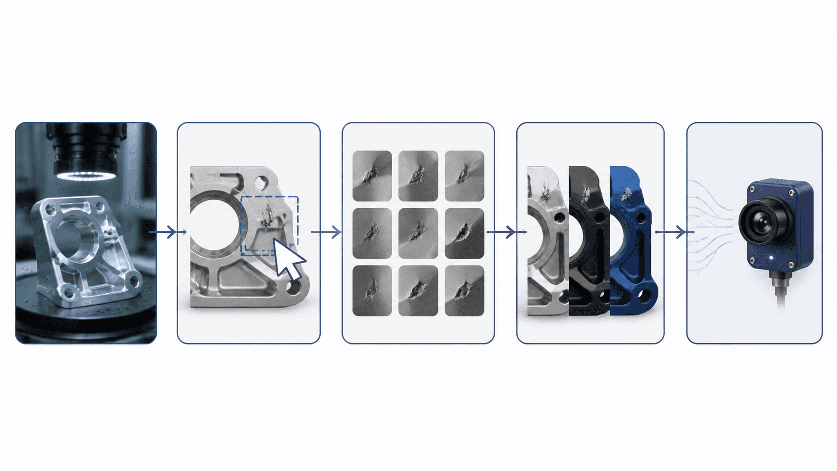
Synthetic defect data, in the manufacturing inspection context, means programmatically generated training images that look like real production images. The base image is real: a high-resolution photo of the manufacturer's actual product, captured by the production camera, under the line's actual lighting. The defect is rendered on top. The combination is a labeled training example.

This is a different proposition from the synthetic data narrative in autonomous vehicles or robotics, where the challenge is simulating an entire visual world. In manufacturing inspection, the system works from a tightly bounded, in-distribution image of the actual product. Synthesis is targeted: place a chip on this edge, a scratch on that surface, a bent pin in that position, a particulate fragment on that fill cavity. Photoshop on rails, run by a quality engineer.

Each synthetic image is generated in under 30 seconds. Three generation tasks run in parallel. For most defect classes, 20 real-image inputs are sufficient to seed the system; the underlying vision model is engineered for sample efficiency, with synthetic generation extending the distribution. More can be used when needed. Sample count stops being a constraint.

Why models do not "go rogue" on synthetic data

The reasonable concern about synthetic training data is whether the model will learn to detect rendered-looking artifacts rather than real defects, and break in production. The answer is engineered into the pipeline rather than assumed.

Real product surface, real camera, rendered defect. Synthetic samples are not generic stock images. Each is built on a real image of the manufacturer's actual product, captured by the actual production camera, under the line's actual lighting profile. The defect is rendered on top. The model trains on real product surface plus realistic defect, not on cartoon artifacts.

Pixel-to-pixel resolution is preserved end to end. The synthetic generation tooling matches the camera's native resolution. There is no upscaling, downsampling, or compression artifact between authoring and deployment.

Direct camera export and import. Models train on synthetic samples in the exact resolution and color space they will see in production, then deploy directly to the smart camera. No format conversion. No domain gap between training and inference.

Engineer-curated output. Every generated sample is reviewed before training. Weak or off-distribution generations are discarded. The training set the model sees is the curated subset, not raw output.

Style Transfer: the variant-fleet multiplier

The most consequential feature inside the synthetic data layer is what we call Style Transfer. Author a defect class once on a known-good image of Variant A. Style Transfer takes that authored defect and renders it onto a clean image of Variant B, in Variant B's actual color, material, plating, weave, and surface finish. The defect physics (shape, scale, severity gradient, location distribution) carry over. The visual context is rebuilt.

The same pass extends to Variants C, D, E, on through the rest of the variant family. Different colors. Different materials. Different geometries. The defect library that took an afternoon to author on Variant A becomes a defect library that covers the entire variant fleet, including variants the line has not yet produced a single unit of.

The practical effect is that the defect library scales sublinearly with the variant count. A 15-variant fleet does not require 15 times the authoring effort of a 1-variant fleet. It requires roughly 1.05 times the effort. Across customer deployments, a single authored defect class reaches an average of 14 variants before any retuning is needed.

The framing this allows is unusual: the model is trained on variants the line has never produced. When a new SKU finally runs the line for the first time, the inspection model already knows what scratches, chips, missing components, and the rest of the defect library look like on it. There is no learning period after SKU launch.

The deployment shape this enables

When the per-variant data step is no longer rate-limiting, HVMM deployments fit into four weeks rather than four quarters.

• Week 1 (pilot). Mount camera. Capture 5 to 20 real images of the highest-volume variant. Generate the synthetic defect distribution for priority defect classes (20 to 30 minutes). Train, deploy, validate against known good and defective samples. Total work: ~4 hours of focused effort across the week.
• Weeks 2 to 3 (expand). Add a recipe per variant. Each variant needs 5 to 20 real images plus a Style Transfer pass (about 6 minutes per variant) plus a training run (38 to 54 minutes). Each variant lands in under 90 minutes of wall-clock work.
• Week 4 (integrate). Connect to the PLC via EtherNet/IP, PROFINET, or Modbus. Automate recipe switching. Configure pass/fail outputs to the reject mechanism. Cut the line over.
• Ongoing (improve). Use Haystack to surface edge cases as production drifts. Retrain individual variant models in minutes when new defect modes appear.

The four-week shape compares against a historical baseline of 11 to 24 months for an equivalently scoped HVMM deployment. The compression is roughly an order of magnitude in calendar time across the full variant fleet.

The limits worth being honest about

Synthetic data is not a universal solvent. Four limits worth naming:

It does not replace base-image diversity. If the captured good-part images do not span legitimate production variation (lighting drift, supplier color drift, surface finish variation across batches), synthetic samples inherit those gaps. The mitigation is unsexy but mandatory: capture good-part images that span the real production envelope, including the edges.

It does not invent defect physics it has not been shown. Genuinely novel failure modes that have never been seen anywhere are not predicted by the synthesis pipeline. They are surfaced by the continuous learning layer (Haystack), not by synthetic generation.

Style Transfer has a fidelity ceiling on extreme material transitions. A defect class authored on matte fabric and transferred to polished metal will require validation. In practice, variant fleets that drive HVMM are usually within-family, but the limit is real.

Regulated environments still require real-data validation. FDA medical device, pharmaceutical, automotive safety-critical, and aerospace applications typically require demonstration of model performance against real production samples regardless of how training data was generated. Synthetic data accelerates the path to a validated model; it does not eliminate the validation step.

Where the bottleneck moves next

For thirty years, the rate-limiting step in industrial vision was per-variant labeled data. With synthetic generation, that step now takes minutes. The next bottleneck up the chain is the rate at which production distributions drift and the rate at which the inspection system absorbs that drift. Drift management is observable, instrumentable, and improvable. Data collection at the variant level was none of those things. Expect the next eighteen months of capability development in this segment to concentrate on the continuous learning layer: faster drift detection, better edge-case surfacing, more autonomous retraining loops.

For the full technical analysis with industry research citations, deployment economics, and reference architecture, see the whitepaper on synthetic data in HVMM manufacturing. For the broader HVMM pattern context, see how AI inspection adapts to your product variants.